
Statistics
Some statistical terms in brief.
Error
Type 1 error (alpha error)
Occurs when the null hypothesis is rejected in a hypothesis test although it is in fact true (based on a randomly increased or lower number of positive results = false positive results).
2Nd type error (beta error)
Occurs when the null hypothesis is incorrectly not rejected in a hypothesis test, although the alternative hypothesis is true.
Probability of error 1st type (alpha risk, producer risk, blind alarm)
Probability of occurrence of an error 1. type.
Probability of error 2nd type (beta risk, consumer risk, omitted alarm)
Probability of occurrence of a 2nd type error.
Coefficient of determination R²
The coefficient of determination R-squared indicates what percentage of the variation in the dependent variable can be explained by a regression model.
It measures the quality of the fit of the model to the data, i.e. how well the independent variables of the model explain the variance (dispersion) of the dependent variable.
Scale:
Between 0 (0 %) and 1 (100 %)
Interpretation:
0 (0 %): Data points are far away from the regression line; model explains the variance poorly. The independent variables do not explain the variance of the dependent variable.
1 (100 %): Data points are close to the regression line. The independent variables explain the entire variation of the dependent variable.
Bonferroni correction
The Bonferroni correction can limit errors of the first type (false positive results) if several statistical tests are carried out simultaneously (multiple testing).
For this purpose, the original significance level (alpha) is divided by the number of tests performed. This results in a stricter significance level that is adjusted for each individual test.
Performing multiple hypothesis tests on the same data increases the probability that a result will be false-positive by chance (falsely interpreted as significant).
The Bonferroni correction prevents this “alpha error accumulation” and prevents an increase in the overall probability of at least one type 1 error above the originally defined level (e.g. 5 %).
Calculation:
Original alpha level (usual: 0.05 = 5 %) for individual test divided by the number of individual tests performed with the same data.
A result is only considered statistically significant if the calculated p-value of the individual test is less than or equal to the newly calculated, adjusted alpha level.
Variables
Nominal scaling
Value contains word / name (“Nomen”), e.g. question about profession.
Dichotomous values
Value with max. 2 values, e.g. yes / no.
Ordinal scaling
Descending or ascending Order of priority (“Order”), not necessarily with equal spacing.
T-value
Difference between two sample means, expressed in units of standard error.
Z-score / Z-value
Distance of a data point from the mean value of the data set, given in standard deviations.
Standard deviation
Root of the average of the squared distance of the data points from the mean value.
In other words:
- Deviation from the mean x deviation from the mean is calculated for each data set (test subjects)
- This value is totaled from all data records (test subjects)
- The root is formed from the result
Measure of the dispersion of the data around the arithmetic mean.
Unit: Like measured values.
Interpretation:
Small standard deviation: The data points are close to the average. Large standard deviation: The data is widely scattered.
Area of application:
Values that have at least interval scale level, i.e. can form a mean value.
Forecast values
Sensitivity
Sensitivity is the counterpart to the false-negative rate. The false negative rate plus sensitivity equals 100%.
The false positive rate is therefore 1 minus sensitivity.
Sensitivity here is therefore the measure of how many people with ADHD are correctly identified as having ADHD.
Specificity
Specificity: Probability that patients without the disease have a negative test result (true-negative rate).
Specificity is the measure of how many healthy people are correctly identified as healthy.
ROC
ROC curve: Receiver operation characteristics curve
The ROC curve is the graphical representation of the true-positive results (number of true-positive results or subjects with disease) compared to the false-positive results (number of false positives or subjects without disease) for a range of cut-off values. The ROC curve graphically shows the intersection between sensitivity and specificity when the cut-off value is adjusted:
- y-axis represents true-positive quantity
- x-axis represents the false-positive quantity
AUC
Area under the curve (AUC).
The larger the area under the ROC curve, the better the test distinguishes between test subjects with and without illness.
Selectivity. 0.5 (= 50 %) = coincidence; 1 (= 100 %) = perfect
Interpretation:
0.5: Coincidence
0.6 - 0.7: poor
0.7 - 0.8: acceptable
0.8 - 0.9: good
0.9 - 1.0: excellent
Correlation
Correlation vs. causality
A correlation is a prerequisite for causality, but does not mean that causality exists.
Example: In children, height correlates strongly with mathematical knowledge, but is by no means causal. There is a “spurious correlation”, although spurious causality is meant, because correlation does exist.
If experiments are designed in such a way that only one variable is changed, this can allow a statement to be made about causality.
In the example with height and math skills, children of the same age and weight in the same grade of the same type of school could be compared with each other. It is foreseeable that height would then no longer correlate with math skills and consequently could not be causal.
The calculation of partial correlations also allows this without leaving all other variables unchanged.
Pearson correlation coefficient (r, product-moment correlation coefficient)
- Sum of the cross products of all test subjects. More precisely: Sum of the values of all test subjects from the deviation of the values of one test subject from the mean value of all test subjects on the X-axis times the same value on the Y-axis.
- Covariance: the determined value is divided by the number of test subjects. This makes the value independent of the number of test subjects,
- Covariance is divided by the product of the standard deviations of Y and X. This makes the value independent of the unit of measurement used and therefore comparable across different test settings.
Identifier: r
Area of application:
- Values that are at least interval scale level
- for metric characteristics, if a linear relationship is assumed
Interpretation:
r = - 1: perfect negative correlation
r = - 0.5 and higher: high negative correlation
r = - 0.3: mean negative correlation
r = - 0.1: low negative correlation
r = 0: no correlation
r = 0.1: low positive correlation
r = 0.3: medium positive correlation
r = 0.5 and higher: high positive correlation
r = 1: perfect positive correlation
Chi-square, χ2
Measures the strength of the correlation between nominally scaled characteristics.
Identifier: χ2
Interpretation:
χ2 = 0: no correlation at all
Upper value is unlimited
Phi-coefficient for correlation of dichotomous values
Phi-coefficient = square root of (chi-square / number of values)
Calculation from four-field table
| X: no | X: yes | |
|---|---|---|
| Y: no | A | B |
| Y: yes | C | D |
Phi-coefficient = (A x D - B x C) divided by the square root of ((A + B) x (C + D) x (A + C) x (B + D))
Phi normalizes the chi-square coefficient to values between 0 and 1, which makes the results comparable.
Area of application:
- dichotomous values (value with max. 2 values, e.g. yes / no)
- only applicable in the case of a four-field table (2 × 2 table)
Interpretation:
Phi = 0: no correlation
Phi = 0.1: low correlation
Phi = 0.3: medium correlation
Phi = 0.5 and higher: high correlation
Phi = 1: perfect correlation
Cramer’s V
Cramer’s V measures the strength of the correlation between nominally scaled characteristics.
Calculation:
- Chi-square is divided by (number of measured values times [minimum number of rows and columns in the crosstab minus 1])
- The root is taken from the result
Lower value: 0 (no correlation)
Upper value: 1 (maximum correlation)
Area of application:
- Crosstabs with at least 2 x 2 fields
Spearman’s Rho
Other names: Spearman correlation, Spearman rank correlation, rank correlation, rank correlation coefficient
Purpose:
Measuring the correlation of rankings
Calculation:
Rho = 1 - (6 × sum of squared rank differences) / (number of data records × [number of data records x number of data records - 1]).
Area of application:
- at least one of the two characteristics is only ordinal scaled and not interval scaled
or - for metric characteristics, if no linear correlation is assumed (the Pearson correlation coefficient is suitable for a linear correlation).
Interpretation:
Rho = - 1: perfect negative correlation
Rho = - 0.5 and higher: high negative correlation
Rho = - 0.3: medium negative correlation
Rho = - 0.1: low negative correlation
Rho = 0: no correlation
Rho = 0.1: low positive correlation
Rho = 0.3: medium positive correlation
Rho = 0.5 and higher: high positive correlation
Rho = 1: perfect positive correlation
Kendal’s Dew
Other names: Kendall’s rank correlation coefficient, Kendall’s τ (Greek letter tau), Kendall’s concordance coefficient
Purpose:
Measurement of the correlation of ordinal-scaled values (rankings)
Calculation:
Tau = (concordant pairs - discordant pairs) / (concordant pairs + discordant pairs)
Area of application:
- Data does not have to be normally distributed
- Both variables must only have an ordinal scale level
- better than Spearman’s Rho when very few data with many rank ties are available
Interpretation:
Tau = - 1: perfect negative correlation
Tau = - 0.8: high negative correlation
Tau = - 0.5: medium negative correlation
Tau = - 0.2: low negative correlation
Tau = 0: no correlation
Tau = 0.2: low positive correlation
Tau = 0.5: medium positive correlation
Tau = 0.8: high positive correlation
Tau = 1: perfect positive correlation
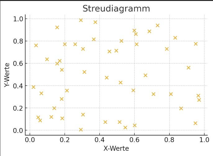
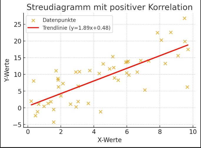
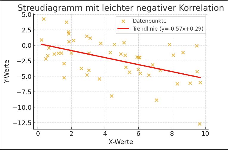
Scatter diagrams
The following scatter diagrams illustrate how data points and trend lines look in different correlation patterns.
No correlation:
Medium positive correlation:
Slightly negative correlation:
Consistency
Cronbach’s alpha coefficient (α)
Cronbach’s alpha measures the internal consistency of a scale or test.
It indicates how well a group of questions (items) captures a single, latent construct and how reliable the scale is overall. A higher alpha value, between 0 and 1, indicates better internal consistency.
Interpretation:
0.60 - 0.67: Poor or questionable internal consistency; the items should possibly not be summarized.
0.70 - 0.79: Acceptable internal consistency.
0.80 - 0.89: Good internal consistency.
from 0.90: Excellent internal consistency.
Cronbach’s alpha increases with the number of items in the scale, which can distort the results.
Use: The items should
- fit together in terms of content
- have the same direction (otherwise recoding is required)
- should have a similar range of values.
Regression
Linear regression
Linear regression is used to predict a dependent variable with the help of one or more independent variables using a linear model.
Linear regression estimates the coefficients for a linear equation that represents a straight line (for multiple variables: surface) that minimizes the discrepancies between predicted and actual values, often using the least squares method.
Simple linear regression: Uses only one independent variable to explain the dependent variable.
Multiple linear regression: Uses several independent variables to explain the dependent variable.
Dependent variable: The variable to be predicted.
Independent variable(s): The variable(s) used for prediction.
Linear model: A model that assumes a linear relationship between the variables.
Least squares method: A calculation method to find the best fitting line by minimizing the sum of squared errors.
Goals and applications:
Causal analysis: Investigating whether and to what extent a dependent variable is related to an independent variable.
Impact analysis: Understanding how the dependent variable changes when the independent variable(s) change.
Prediction: Prediction of values of the dependent variable based on the values of the independent variables.
Prerequisites:
Variables have a linear relationship to each other.
The dependent variable is at least interval scaled.
Few outliers in the data, as outliers can strongly influence the results.
Logistic regression
Logistic regression is used to predict the probability of a binary event (e.g. yes/no, success/failure) as a function of one or more independent variables.
While linear regression predicts continuous values, logistic regression uses the sigmoid function (inverse logit function) to generate an s-shaped curve that provides probabilities between 0 and 1.
Logistic regression is often used for classification (e.g. fraud detection based on data patterns or disease prediction based on factors such as age, smoking, gender, etc.).
Result: categorical variable with two possible values (binary dependent variable).
The factors influencing the probability of the result (independent variables) can be numerical or categorical.
Logistic function (sigmoid): This function maps the relationship between the independent variables and the binary dependent variable. It converts a linear combination of the input features into a probability value between 0 and 1.
Prediction of probability: The model estimates the probability that an observation belongs to one of the two categories.
ANOVA
ANOVA (Analysis of Variance) is used to test for significant differences between the mean values of more than two groups.
ANOVA is an extension of the t-test, which only compares two groups. ANOVA compares the variance between three or more groups with the variance within the groups to determine whether the differences in the group means are statistically significant.
Calculation:
F-ratio = variance between the groups divided by variance within the groups.
Interpretation:
The higher the F-ratio, the greater the differences between the groups compared to the random differences within the groups.
One-factorial ANOVA
Examines the influence of a single independent variable on a dependent variable.
Multi-factorial ANOVA
Examines the influence of two or more independent variables.
MANOVA
MANOVA (multivariate analysis of variance) is used to analyze deviations between two or more groups when there are several dependent variables.
Target:
To determine whether the mean values of the dependent variables differ significantly between the groups, taking into account the interrelationships between the variables.
ANCOVA
ANCOVA (analysis of covariance) is a statistical method for analyzing covariance. ANCOVA combines analysis of variance (ANOVA) with linear regression.
In contrast to ANOVA, ANCOVA takes into account a further metric variable, the covariate, in addition to the independent variable.
Target:
Investigation of the influence of one or more independent variables on a dependent variable by eliminating the effect of one or more covariates (confounding variables).
Example:
Study of different stimulants (independent variable), controlling for caffeine intake (covariate), to compare the frequency of drug side effects (dependent variable).
MANCOVA
Mancova (Multivariate Analysis of Covariance) is a statistical method for analyzing the difference in the mean values of several dependent variables between different groups while simultaneously controlling for the effects of one or more covariates (confounding variables).
Mancova is an extension of Manova (multivariate analysis of variance) and Ancova (analysis of covariance), which makes it possible to analyze several dependent variables at the same time and simultaneously eliminate interfering influences of covariates.
Effect size
Mean value difference, SMD, Cohens’ d
Serves to neutralize the influence of different scales and thus make tests comparable.
Calculation:
(mean value of change with verum minus mean value of change with placebo) divided by (pooled) standard deviation
Interpretation:
Cohen’s d to 0.2: very small, can only be determined statistically
Cohen’s d 0.2 to 0.5: small
- recognizable on the individual from 0.5
Cohen’s d 0.5 to 0.8: medium
Cohen’s d from 0.8: strong
Beta coefficient
Beta coefficient is the regression coefficient after conversion (standardization) of the dependent variable and independent variables into z-values.
Used to calculate the Effect size in regression analyses.
Interpretation:
Beta coefficient to 0.1: very small
Beta coefficient 0.1 to 0.3: small
Beta coefficient 0.3 to 0.5: medium
Beta coefficient from 0.5: strong
Probability
Odd Risk (OR)
Ratio of two “odds” (probability of success divided by probability of failure).
Often used in case-control studies to measure the association between an exposure (e.g. smoking) and an outcome (e.g. lung cancer).
Hazard Risk (HR)
Ratio of the so-called “hazard rates” (current risk of an event in a certain period of time) between two groups.
Used in particular in survival time analyses to investigate the effects of treatment on the time until the event (e.g. death).
P-value
Interpretation:
- p < .05* Significant
- p < .01** Highly significant
- p < .001*** Highly significant
Number needed to…
Number needed to treat, NNT
The number needed to treat (NNT) is the statistically necessary number of treatments that achieve an additional positive outcome compared to an alternative treatment (usually placebo or waiting list). NNT is calculated as the reciprocal of the absolute risk reduction.
For example, if the percentage difference between the proportion of responders in the active group and in the placebo group is 11 percentage points, the reciprocal value 9 is the NNT.1
Number needed to harm, NNH
Number of treatments required to trigger an adverse reaction.
Number needed to screen, NNS
Number of screening procedures required to avoid a risk (death, adverse event).
Online statistics calculator
While specialized programs are used for professional statistical evaluations (MATLAB, Statistica, SPSS or even free software such as PSPP, R, gretl)23 , which are far more powerful than Excel, there are also some online calculators that enable simple statistical analyses.
Numiqo online calculator Descriptive statistics:
- Hypothesis test
- Chi-square test
- T-test
- Dependent t-test
- ANOVA
- Three-factorial ANOVA
- Mixed ANOVA
- Mann-Whitney U-test
- Wilcoxon test
- Kruskal-Wallis test
- Friedman test
- Binomial test